PART 2: Applications
2.1 Image "Sharpening" (Unsharp Masking)
Image sharpening amplifies high spatial frequencies using the unsharp mask equation: \(I_{\text{sharp}} = I + \alpha (I - I * G)\), where \((I - I * G)\) isolates high-frequency details (by subtracting the blurred image from its original non-blurred form). I tested this on the Taj Mahal and custom test images across varying values of \(\alpha\).
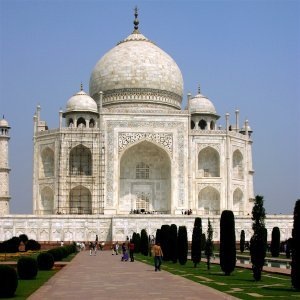
Figure 1a. Original image of Taj Mahal
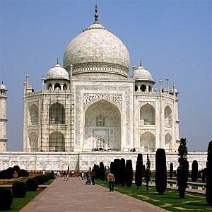
Figure 1b. Image of Taj Mahal sharpened α = 1.0
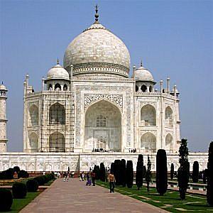
Figure 1c. Image of Taj Mahal sharpened α = 1.5
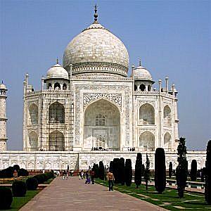
Figure 1d. Image of Taj Mahal sharpened α = 2.0
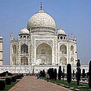
Figure 1e. Image of Taj Mahal sharpened α = 5.0

Figure 1f. Original image of road
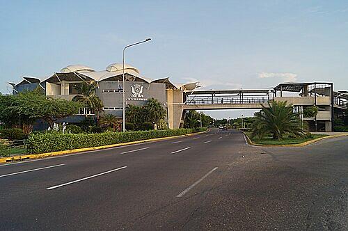
Figure 1g. Image of road sharpened α = 1.0
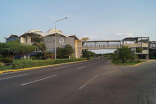
Figure 1h. Image of road sharpened α = 1.5
Evaluation Experiment: Sharp → Blur → Re-sharpen
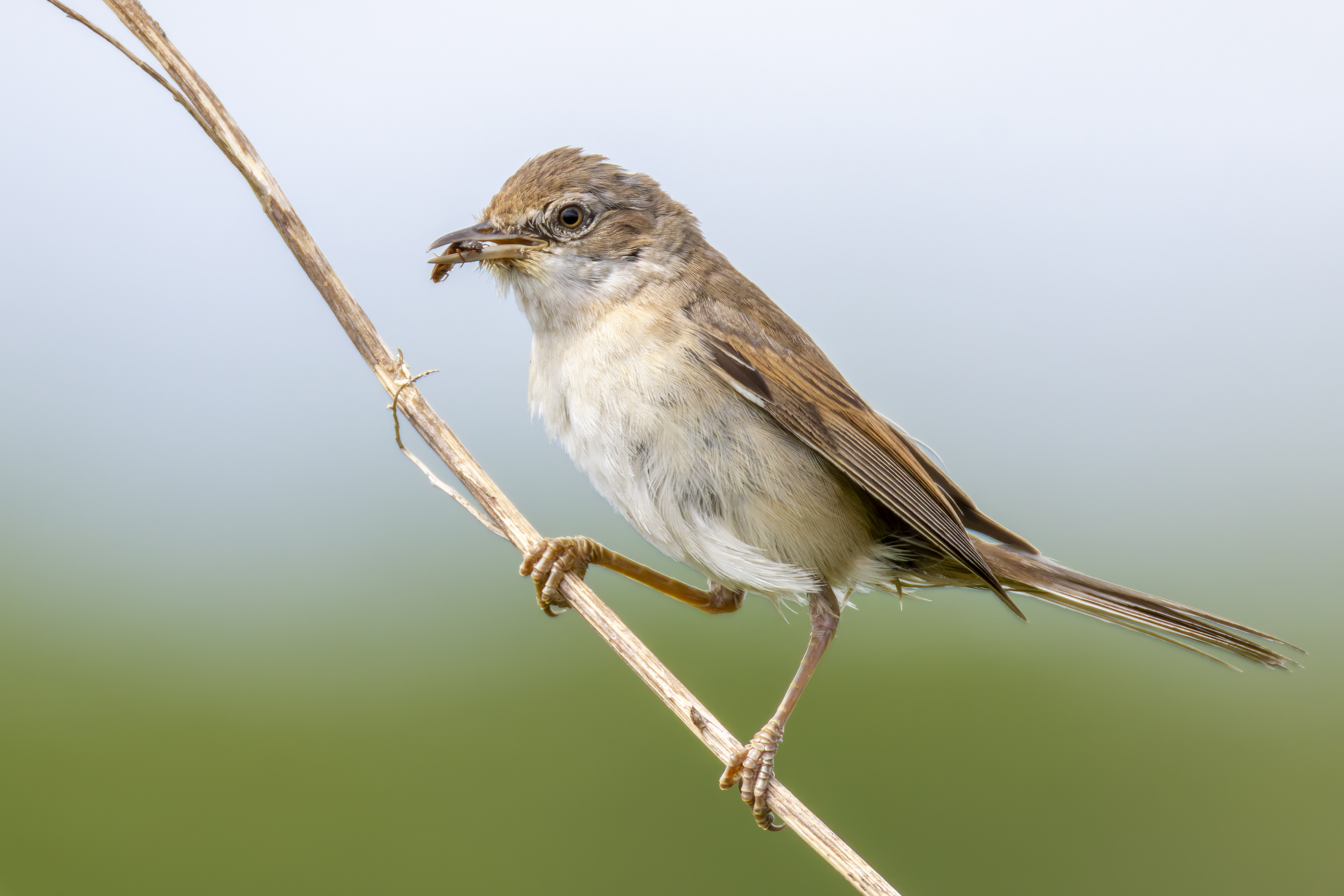
Figure 1i. Original image of bird
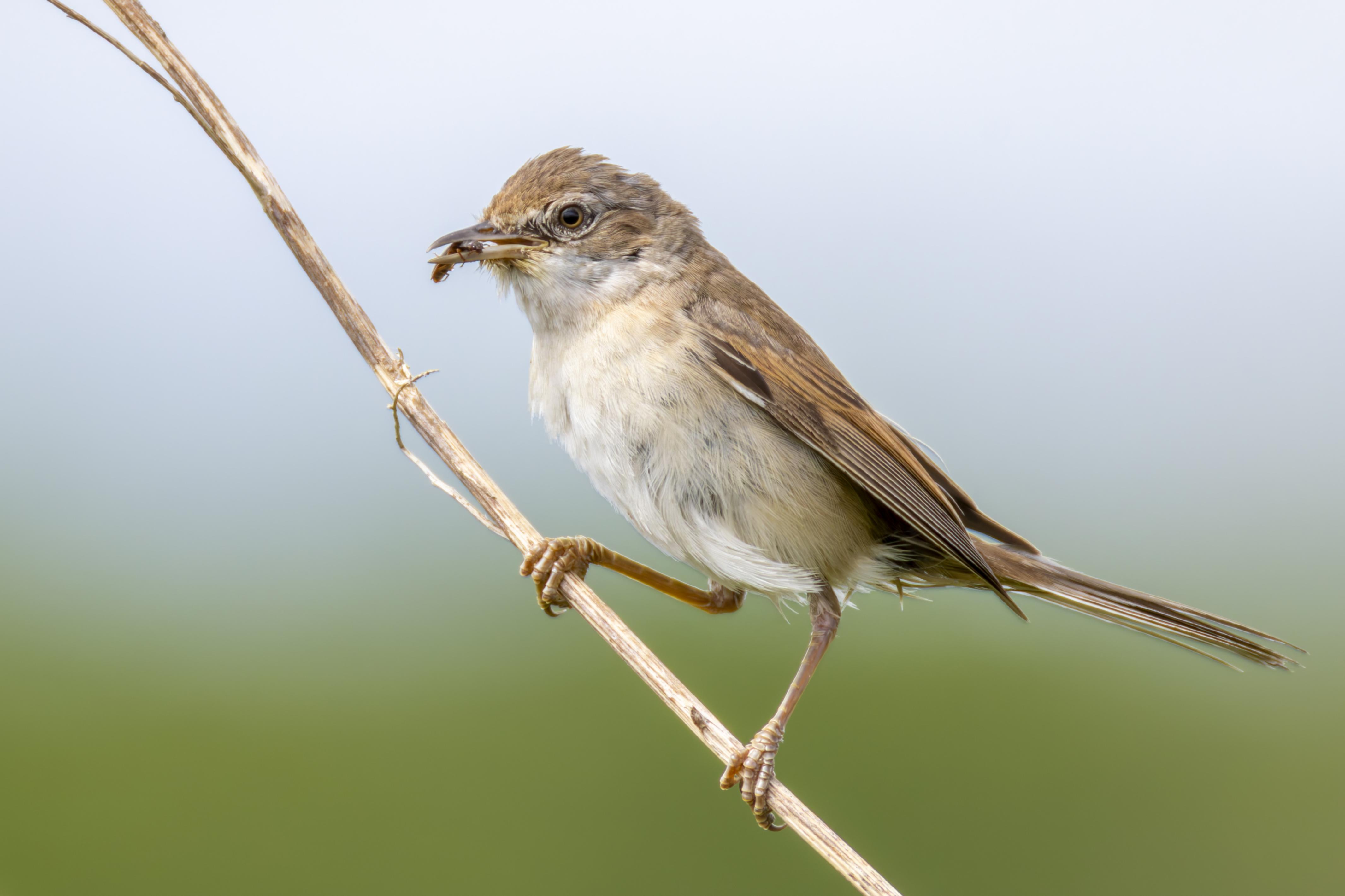
Figure 1j. Blurred image of the bird Blurred (G * I)
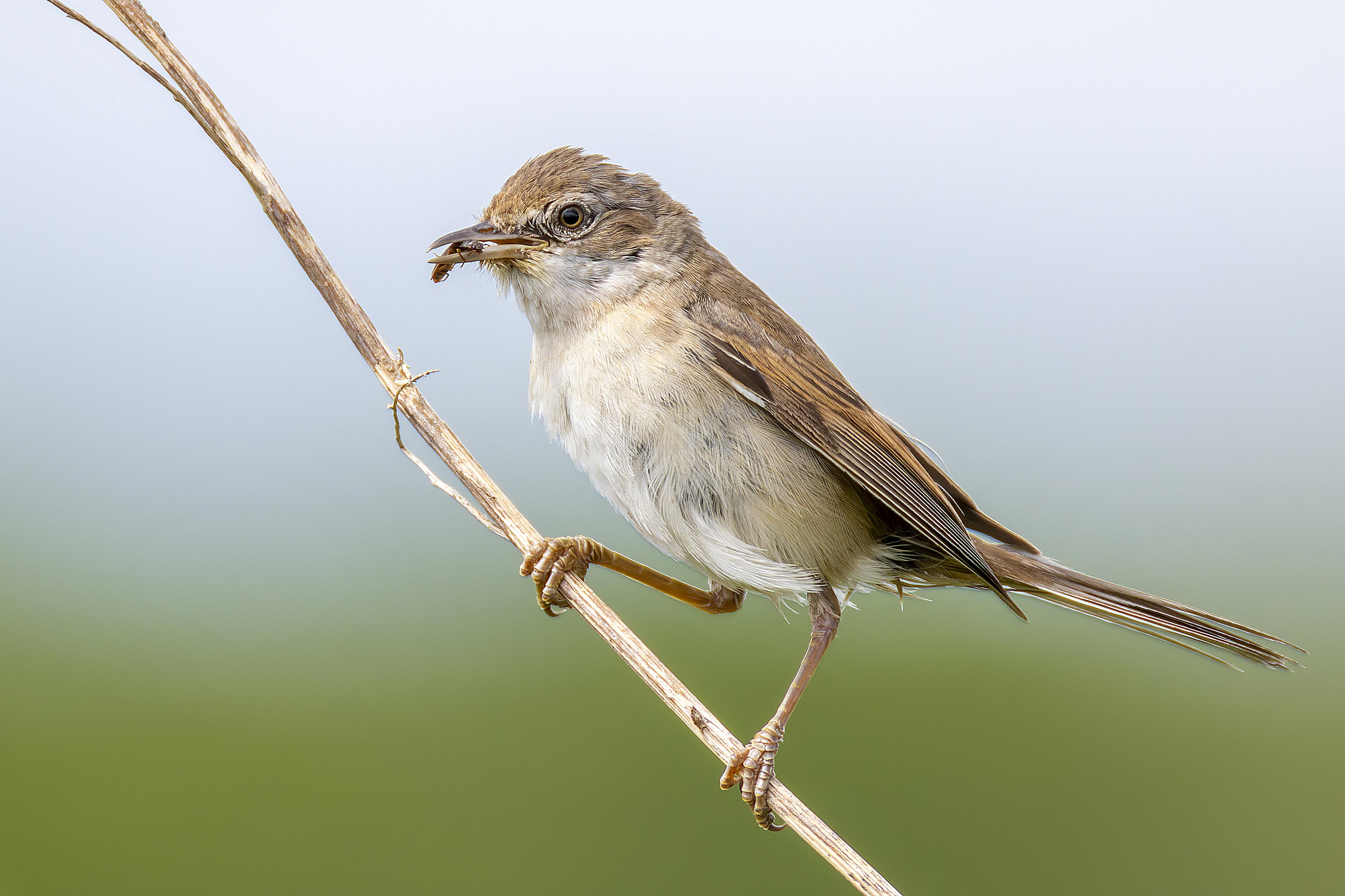
Figure 1k. Image of bird re-sharpened α = 2.0
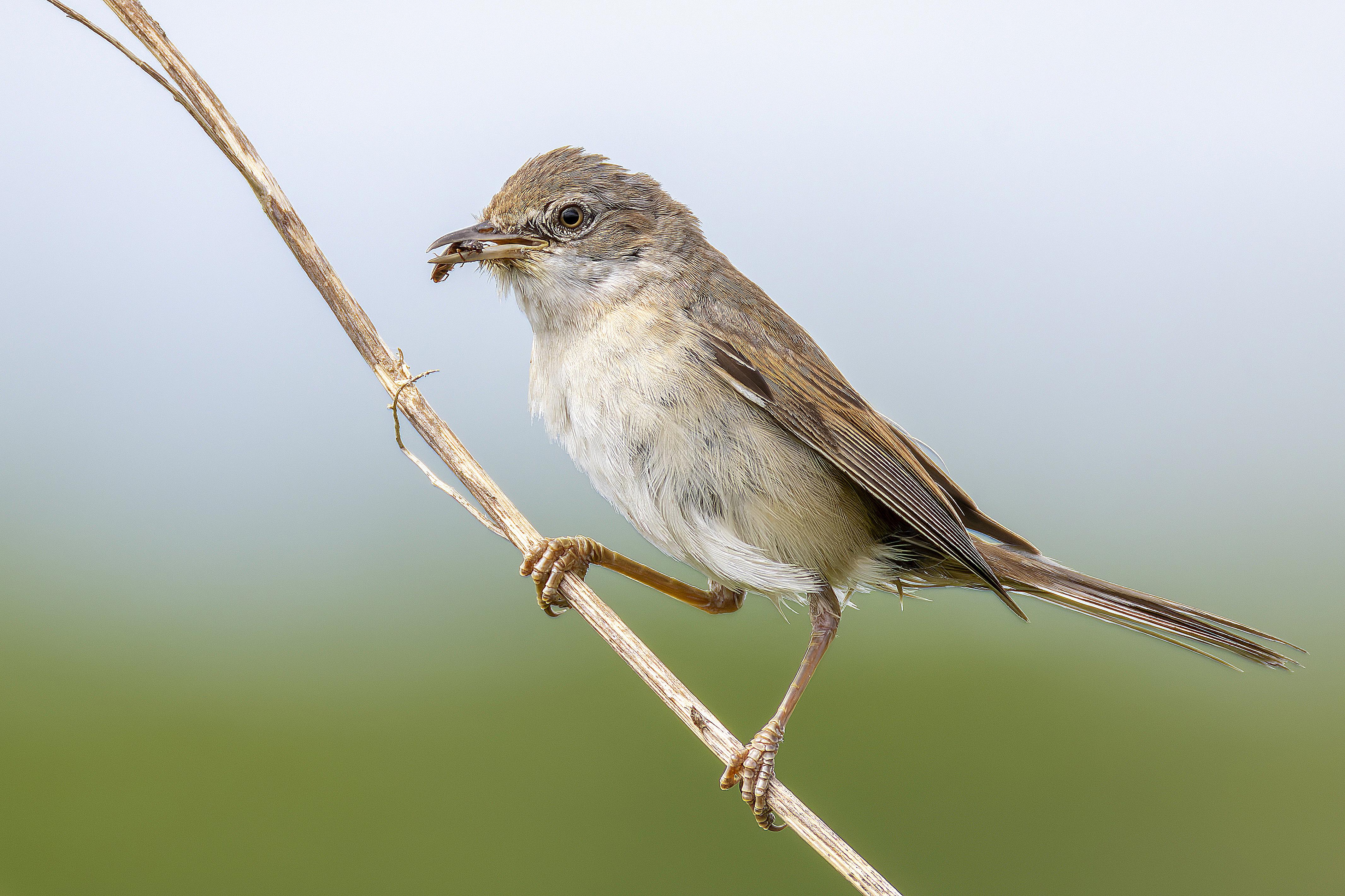
Figure 1l. Original image of bird sharpened α = 10.0
Evaluation & Color Troubleshooting Insights:
- Blur vs. Resharpen: Re-sharpening a blurred image recovers visible edge contrast, but it cannot fully restore lost high-frequency information. Frequencies destroyed by Gaussian blurring are permanently lost; unsharp masking simply boosts whatever residual gradients remain, leading to slight halo artifacts around strong edges.
- The Color Mystery at Extreme α = 10.0: When pushing \(\alpha\) to extreme values, colors appear washed out or severely discolored. This occurs because extreme scaling causes severe RGB pixel clipping which drives values beyond \([0.0, 1.0]\) so individual color channels hit pure black or pure white, destroying color saturation (this can be observed in when comparing Figure 1i- birds original image- to Figure 1i- the bird's image sharpened with α = 10.0).
2.2 Hybrid Images & Frequency Analysis
Hybrid images (Oliva, Torralba & Schyns, SIGGRAPH 2006) combine the low spatial frequencies of Image A with the high spatial frequencies of Image B. When viewed up close, high frequencies dominate human perception however, from a distance, high frequencies blend away and low frequencies take over.
I built alignment tools using similarity transforms based on clicked eye coordinates and tested 3 pairs: Derek + Nutmeg (given in assignment), football players Cristiano Ronaldo + Mohammed Salah, and main characters of the Netflix series: Saul Goodman from Better Call Saul and Walter White from Breaking Bad.
Full 5-Stage Fourier Transform Pipeline (BBCS: Saul Goodman + Walter White)
Below is the 2D Fourier log-magnitude spectrum (np.log(np.abs(np.fft.fftshift(np.fft.fft2(img))))) tracked across every stage of the hybrid pipeline:
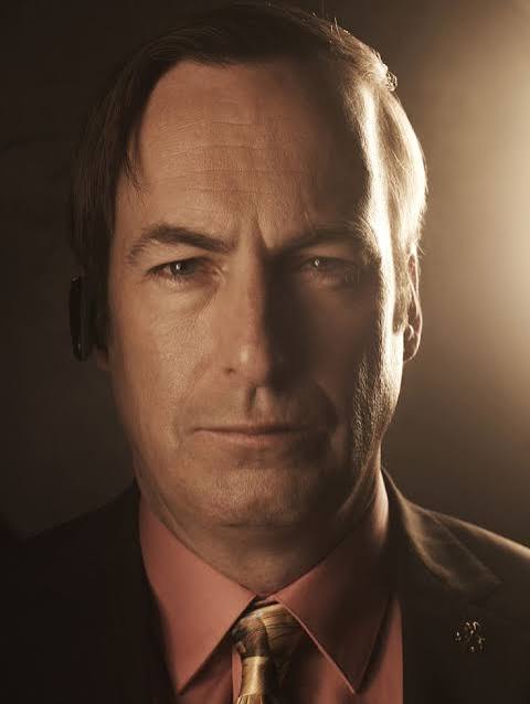
Figure 2a. Saul Goodman original image
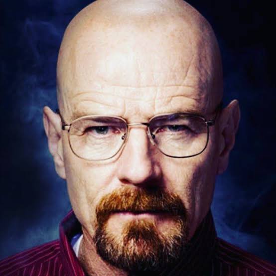
Figure 2b. Walter White original Image
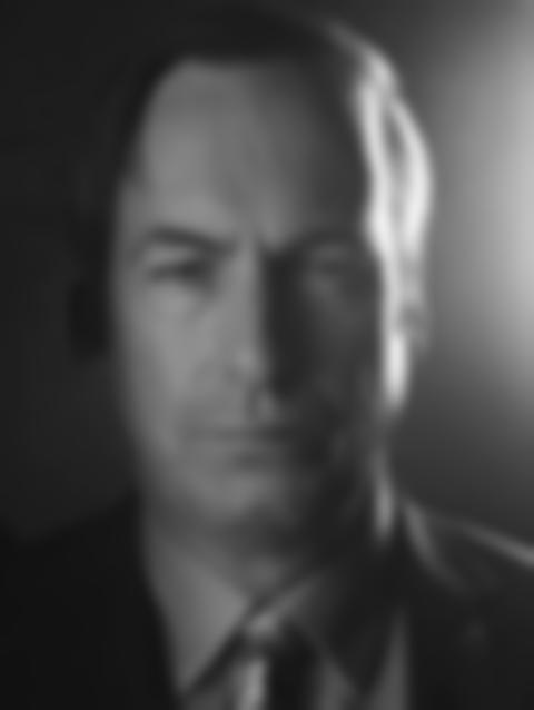
Figure 2c. Low pass filter on Saul
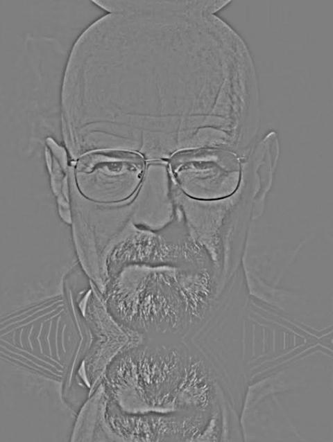
Figure 2d. High pass filter on Walter White
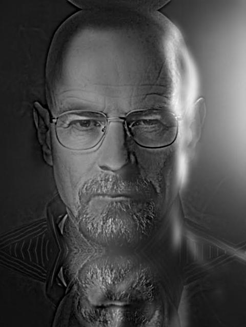
Figure 2e. Hybrid result
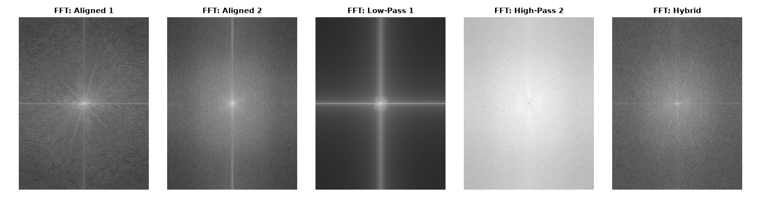
Figure 2f. 2D Fourier log-magnitude spectrum
FFT Spectrum Analysis:
- Stage 1 & 2 (Inputs): Bright central cross indicates that natural images concentrate most energy in low frequencies.
- Stage 3 (Low-Pass): Outer high-frequency regions are completely blacked out after Gaussian blurring.
- Stage 4 (High-Pass): The central DC cross is attenuated, leaving energy concentrated in outer high-frequency rings.
- Stage 5 (Hybrid): Combines the bright central low-pass core of Saul with the outer high-pass detail ring of Walt.
Additional Hybrid Results
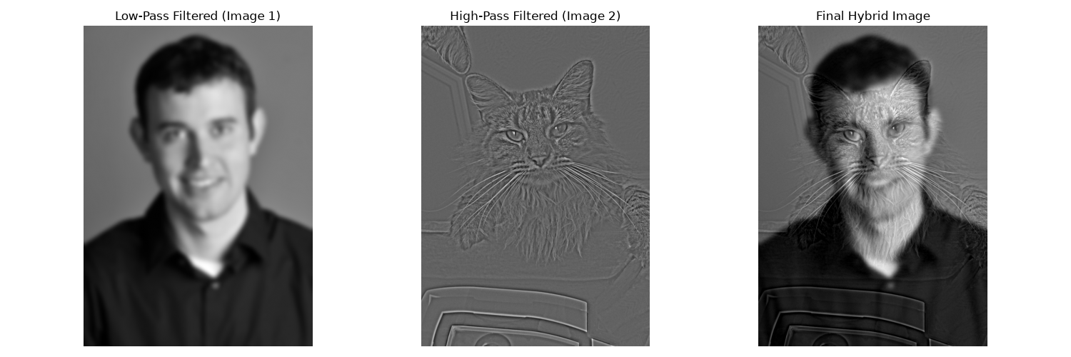
Figure 2g. Derek and Cat hybrid
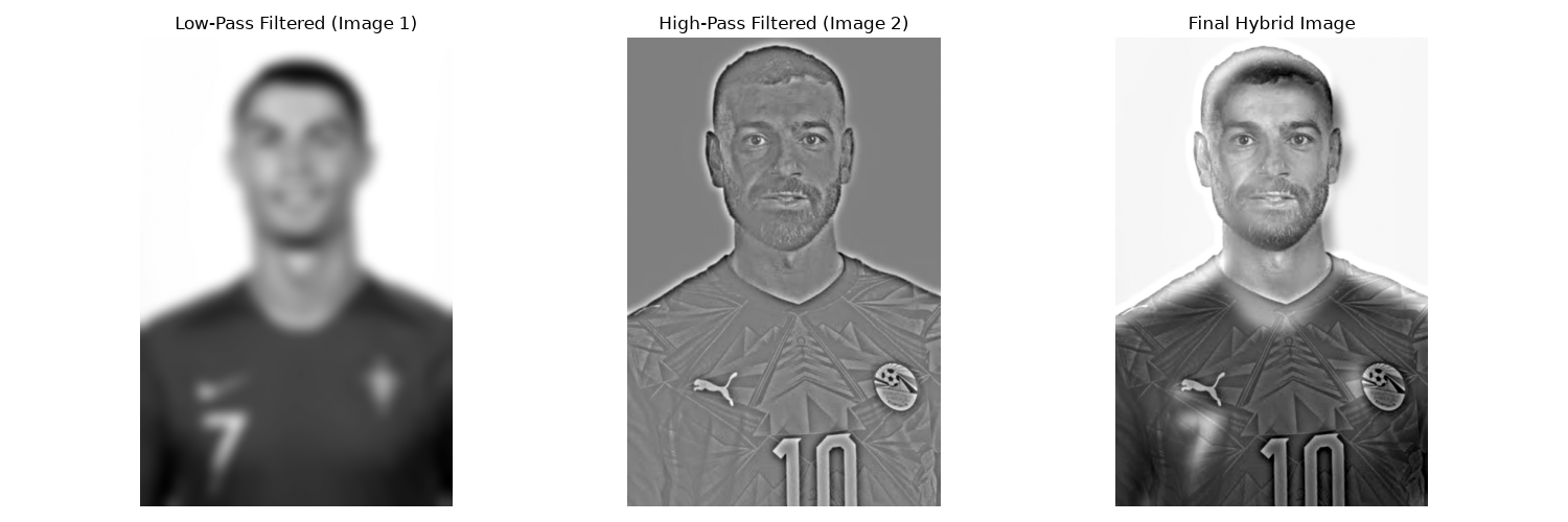
Figure 2h. Cristiano Ronaldo and Mohammed Salah (Footballers)
Bells & Whistles (Part 2): Color Mode Strategy Comparison
I evaluated three color configurations for hybrid generation: color_mode='low', color_mode='high', and color_mode='both'.
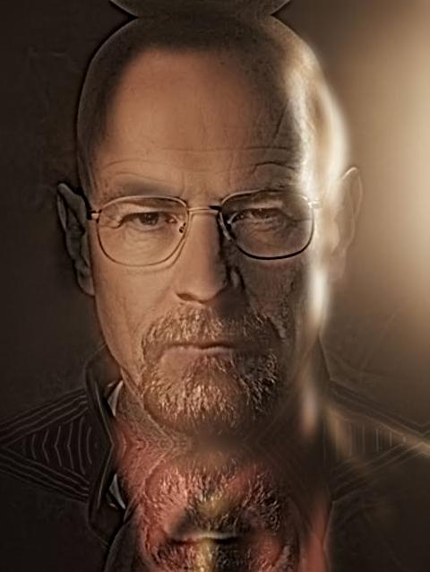
Figure 2i. Color on Low-Pass Only
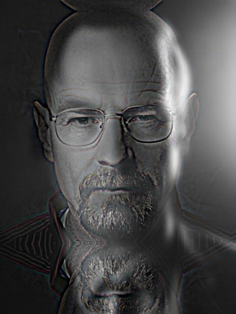
Figure 2j. Color on High-Pass Only
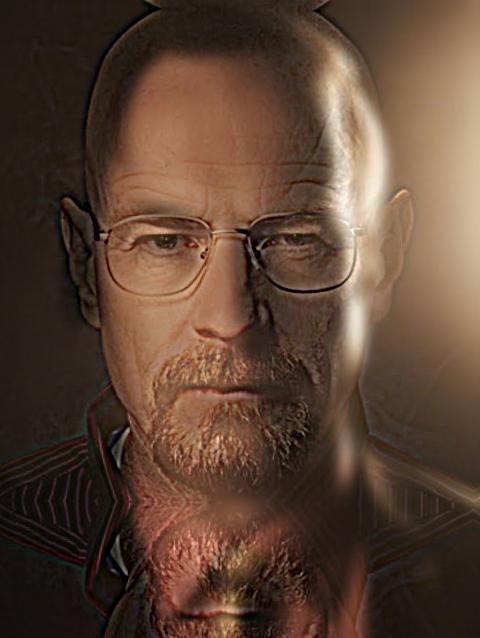
Figure 2k. Color on Both Components
Color Justification: Applying color only to the low-frequency component (color_mode='low') produces the best perceptual result. Human vision perceives broad color saturation in low spatial frequencies, whereas high-frequency color introduces chromatic noise that disrupts the perceptual grouping at distance. Color on low-pass blends naturally without giving away the high-frequency illusion up close. From the images above we can see that coloring the low frequency and both high and low frequency images yields same result. So for the good of the computation power I would say applying color to low-frequency component is sufficient.
2.3 & 2.4 Gaussian & Laplacian Stacks & Multiresolution Blending
Unlike pyramids, stacks do NOT perform downsampling. In stacks, every level retains full \(H \times W\) resolution. A Gaussian stack applies progressively larger Gaussians (\(\sigma = 1, 2, 4, 8, 16, 32 \dots\)), and the Laplacian stack computes difference layers \(L_i = G_i - G_{i+1}\), with the coarsest level \(L_{N-1} = G_{N-1}\).
Multiresolution blending (Burt & Adelson 1983, p. 230) blends each Laplacian level using the Gaussian stack of a binary mask \(G_{\text{mask}}\):
\[L_{\text{blend}}[i] = G_{\text{mask}}[i] \cdot L_A[i] + (1 - G_{\text{mask}}[i]) \cdot L_B[i]\]
Szeliski Fig 3.42 / Burt & Adelson Fig 10 (Apple + Orange "Oraple" 4x3 Grid)

Figure 3a. Level 0: Apple Laplacian High Frequencies

Figure 3b. Level 0: Orange Laplacian High Frequencies

Figure 3c. Level 0: Blended High Frequencies

Figure 3d. Level 1: Apple Laplacian Bandpass

Figure 3e. Level 1: Orange Laplacian Bandpass

Figure 3f. Level 1: Blended Bandpass

Figure 3g. Level 2: Apple Laplacian Medium Scale

Figure 3h. Level 2: Orange Laplacian Medium Scale

Figure 3i. Level 2: Blended Medium Scale

Figure 3j. Level 3: Apple Coarse Base Component

Figure 3k. Level 3: Orange Coarse Base Component

Figure 3l. Level 3: Blended Base Component

Figure 3m. Level 4: Apple Coarse Base Component

Figure 3n. Level 4: Orange Coarse Base Component

Figure 3o. Level 4: Blended Base Component
Stack Performance Note:
Running a 6-level full-resolution stack required 2 minutes 39 seconds
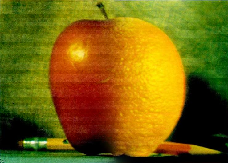
Figure 3p. 6-Level Laplacian Stack Blend (σ0 = 1.0)

Figure 3q. 7-Level Laplacian Stack Blend (σ0 = 1.0)
Custom Blends with Straight and Irregular Masks
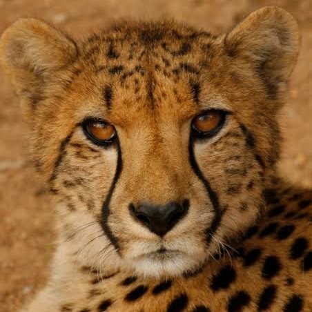
Figure 3r. Cheetah original image
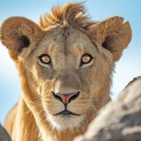
Figure 3s. Lion original image
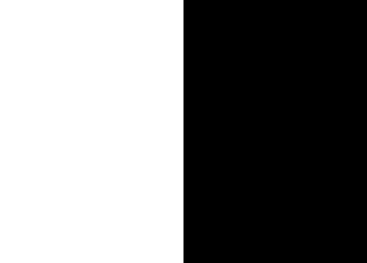
Figure 3t. Mask is vertical
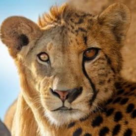
Figure 3t. Cheetah + Lion = Cheeion
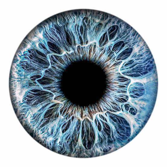
Figure 3u. Eye Original Image
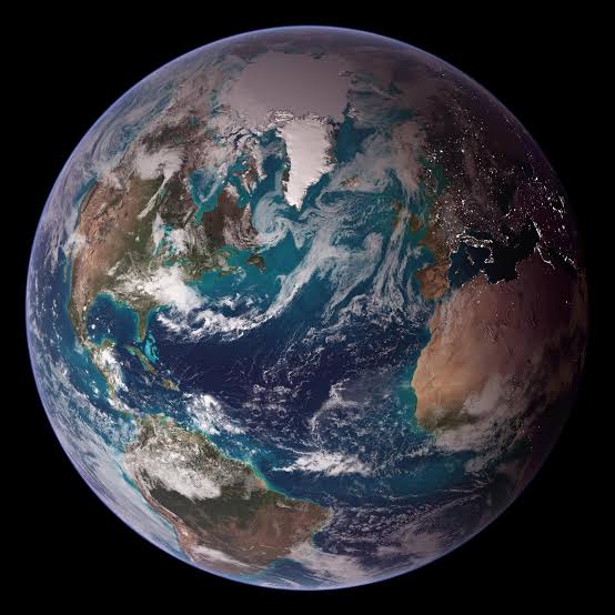
Figure 3v. Earth Original Image
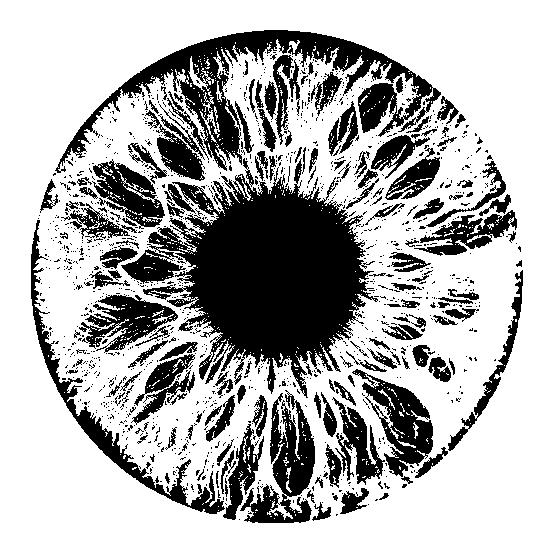
Figure 3w. Irregular Binarized Mask (Threshold = 0.4)
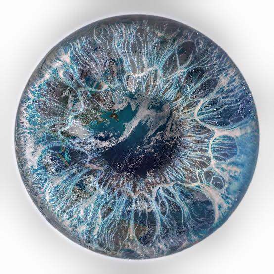
Figure 3x. Eye + Earth = Earth Eye Composite
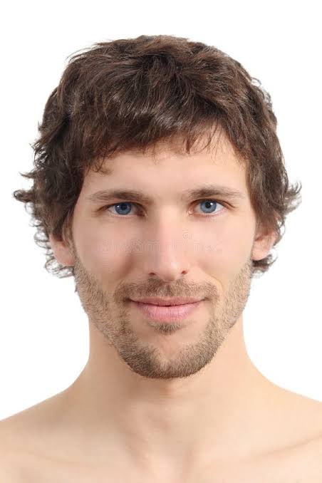
Figure 3y. Man Original Image
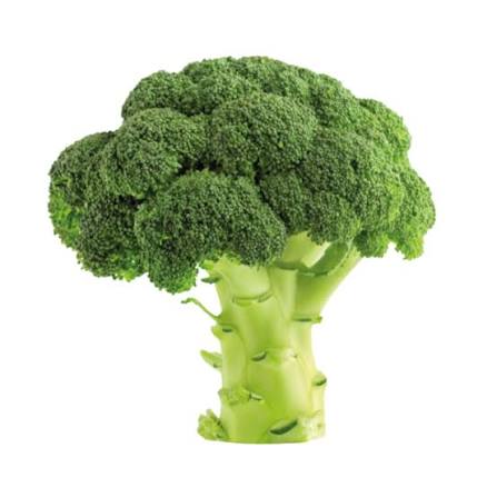
Figure 3z. Broccoli Original Image
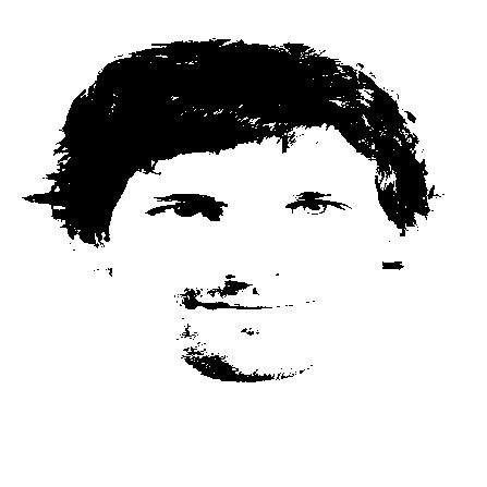
Figure 3aa. Custom Binarized Threshold Mask (Threshold = 0.4)
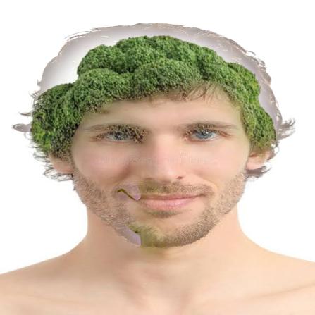
Figure 3ab. Man + Broccoli = Brocco-Man Composite
Bells and Whistles
Mask Choice & Color Justification for Blending: For the Eye + Earth blend, I thresholded the grayscale eye image at 0.4 to isolate the pupil/iris geometry. Using full-color Laplacian stacks allows high-frequency skin textures and earth clouds to seam tightly while low-frequency lighting smoothly transitions across the irregular boundary without harsh boundary seams.